LLM energy efficiency is not a fixed model trait. The same model can consume very different energy per useful request when you change prefill length, output length, batch shape, precision, request timing, GPU clocks, or the serving runtime. Measure those factors with latency and quality before you call one setup efficient.
This guide is for advanced readers who operate or evaluate LLM inference. Its practical conclusion is simple: collect energy at the device or node, explain it with serving telemetry, and normalize it against useful work at the request layer. A single watts reading cannot do all three jobs.
The distinction matters more as reasoning budgets grow. Extra generated tokens increase compute, but the system around those tokens decides how effectively the hardware does that work. My earlier analysis of reasoning tokens and their compute cost covers the workload side. This article focuses on the energy audit and serving side.
LLM energy efficiency is a serving-stack result
Energy is power integrated over time. If a GPU averages 400 watts for ten seconds, it uses 4,000 joules. That part is easy. The hard part is choosing the time window, the hardware boundary, and the reporting unit.
“Energy per token” can mean at least three different things:
| Metric | Useful for | What it can hide |
|---|---|---|
| --- | --- | --- |
| Joules per output token | Decode-heavy chat and generation | Prompt processing, failed requests, quality differences |
| Joules per effective input token | Prefill and long-context work | Output work and end-to-end request value |
| Joules per successful request | Product and workload comparison | Large differences in prompt and response length |
| Requests per kilowatt-hour | Capacity and operational planning | Request difficulty, quality, and latency |
None is universally correct. Choose the unit that matches the service contract, then report enough context so another team can repeat the test.
The hardware boundary matters just as much. NVIDIA’s management API exposes device energy counters on supported hardware. That can produce a clean GPU delta, but it does not include CPU work, host memory, storage, networking, cooling, or power-conversion losses by default. CodeCarbon can extend the boundary with measured and estimated parts, yet its docs describe fallback estimates for hardware it cannot read. “Measured by a tool” does not mean every part was metered.
Four studies measured different parts of the stack
Recent research makes the system effect visible. The headline percentages below are not a leaderboard. Each study uses a different platform, workload, baseline, and energy boundary.
| Study | Scope and method | Reported result | Boundary to keep in view |
|---|---|---|---|
| --- | --- | --- | --- |
| AFlex | Disaggregates attention and feed-forward work, then controls provisioning, frequency, batch size, and microbatching on A800 systems | Up to 49% less energy per token than the tested disaggregated baseline while meeting TTFT and TPOT targets | Two model families, A800 hardware, and evaluated production-style traces |
| Festina | Coordinates placement, GPU partitioning, operating point, consolidation, and migration for shared H100 inference | Up to 56% lower energy with SLO attainment kept within two percentage points in the reported setup | Shared-GPU serverless context; gains shrink when prefill is already compute-intensive |
| EnerInfer | Predicts throughput and power across NPU and memory settings, then manages control settings under thermal limits | Energy-efficiency gains of 65% on phones, 12% on a laptop, and 24% on an edge board | End-to-end device savings were smaller, 4.2–11%, because other parts and phases still consumed energy |
| Understanding Efficiency | Tests quantization, batching, arrival patterns, and serving choices on H100 GPUs | Continuous batching cut energy per request by 12.5× versus the study’s sequential baseline; structured arrivals reached larger gains in a fixed test | Short prompts, two Llama model sizes, one accelerator family, and mostly GPU-focused energy data |
The shared result is stronger than any individual percentage: orchestration can move energy use enough to invalidate a model-only estimate. The papers also show why “use lower precision” is incomplete advice. The H100 study found that lower precision helped compute-bound prefill, while dequantization and kernel overhead could erase or reverse the benefit during memory-bound decode.
Treat every “up to” number as a property of the authors’ experiment. AFlex does not prove a 49% saving on your B200 cluster. EnerInfer does not prove a 65% whole-device saving for every phone. The results identify controls worth testing, not savings you can copy into a forecast.
Separate prefill from decode before you optimize
An LLM request has two phases with different bottlenecks.
Prefill is usually compute-heavy
Prefill processes the prompt and builds the key-value cache. Long prompts create bursts of parallel matrix work. Precision changes and higher clocks may help when this phase is compute-bound, but a lower time-to-first-token can still come with a higher power peak. Measure energy, not power alone.
Decode is usually memory-heavy
Decode produces tokens one step at a time. It repeatedly reads model weights and the growing KV cache, so memory traffic and batch formation often dominate. Higher clocks can add power without proportional throughput. Quantization can also add conversion overhead when the kernels or hardware path are not well matched.
This phase split explains why an average over the whole request can mislead. A setup may improve long-prompt prefill and hurt short-prompt decode. Report at least prompt length, output length, batch or concurrency, precision, and phase timings with every energy result.
The KV cache belongs in the same record. My guide to KV cache eviction failures explains the reliability side. For energy work, cache pressure can change memory traffic, recomputation, placement, and retry rates. A run with silent evictions is not comparable to one without them.
Run an energy audit that protects latency SLOs
The audit needs three connected layers: request outcomes, serving context, and device or node energy.
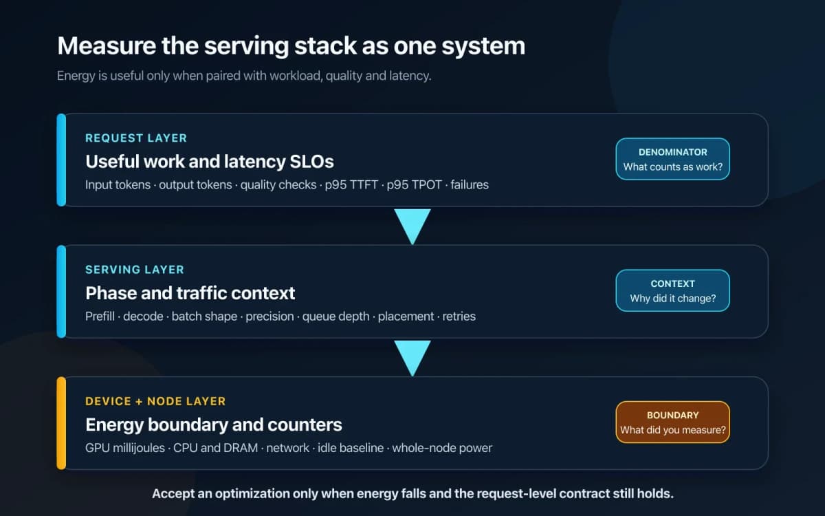
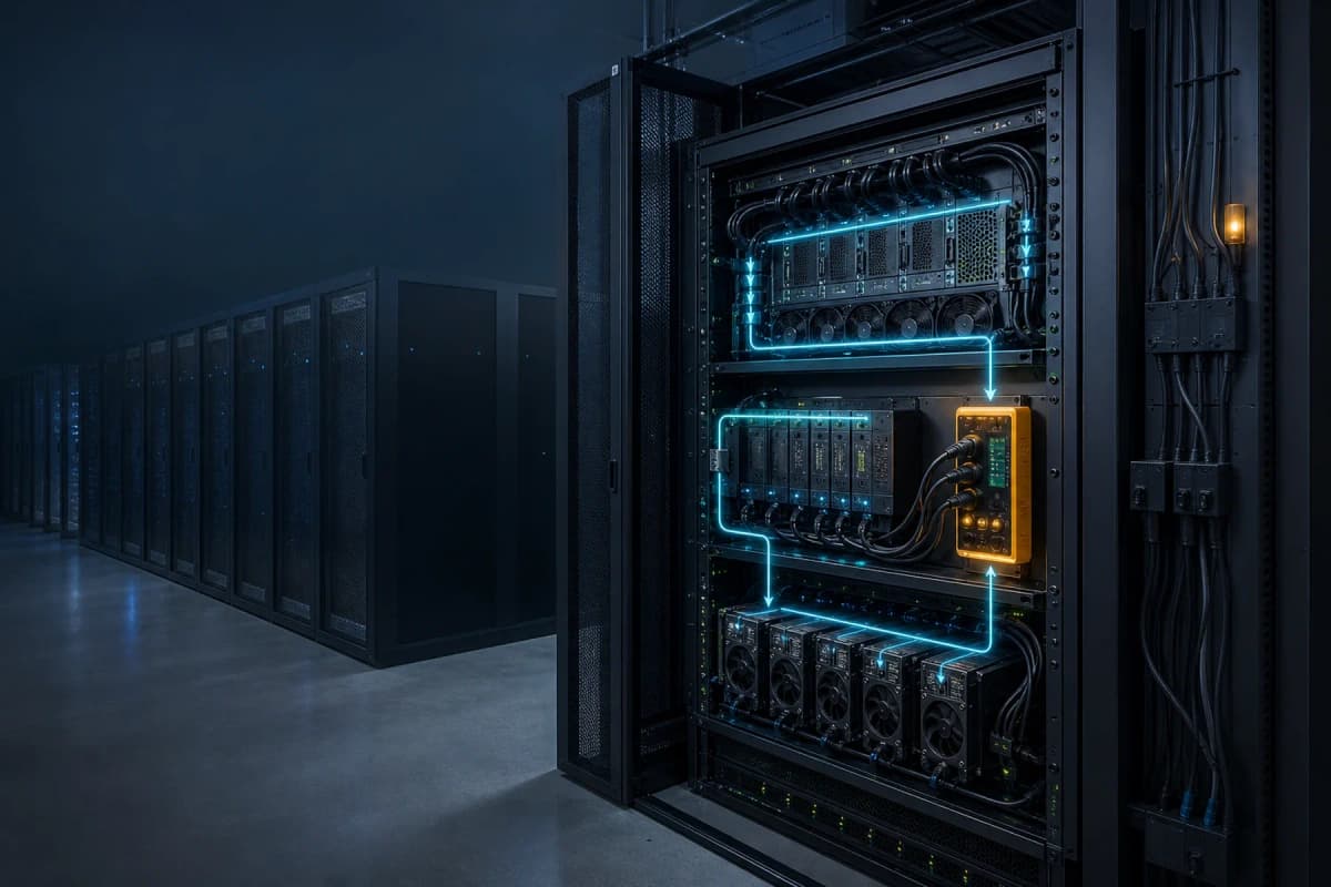
*A useful energy result needs a clear unit, serving context, and an explicit hardware boundary.*
1. Freeze a representative workload
Build workload slices instead of one synthetic average. At minimum, separate short and long prompts, short and long outputs, steady and bursty arrivals, and the quality tiers your application uses. Keep the model, tokenizer, sampling policy, and stopping rules fixed during a comparison.
Use real request shapes when privacy and consent permit. If you use synthetic prompts, preserve the token-length and arrival distributions that drive the system. The final report should label synthetic demand as synthetic.
2. Record request-level outcomes
For every request, capture:
Do not delete failures from the energy total. A setup that spends less energy on completed requests by timing out the hard ones is not more efficient.
3. Record serving context
Log the controls that can explain a change: prefill and decode duration, batch size, active sequences, queue depth, precision, parallelism, cache occupancy, placement, GPU clocks or power limit, and co-tenant load.
This telemetry also catches idle and burst effects. A runtime that keeps CPUs busy while the GPU waits can look fine in a GPU-only reading and worse at the node or fleet boundary. Open-source issue threads are useful for finding these failure modes, but they are anecdotes until you reproduce them on your stack.
4. Measure an explicit energy boundary
On supported NVIDIA GPUs, NVML exposes a total-energy counter in millijoules. A minimal Python probe can bracket a fixed workload:
from pynvml import (
    nvmlDeviceGetHandleByIndex,
    nvmlDeviceGetTotalEnergyConsumption,
    nvmlInit,
    nvmlShutdown,
)

nvmlInit()
gpu = nvmlDeviceGetHandleByIndex(0)
start_mj = nvmlDeviceGetTotalEnergyConsumption(gpu)

run_fixed_workload()  # same requests, model, and stopping rules

end_mj = nvmlDeviceGetTotalEnergyConsumption(gpu)
nvmlShutdown()

gpu_joules = (end_mj - start_mj) / 1_000
joules_per_output_token = gpu_joules / completed_output_tokens
The NVML device query docs define the counter and its units. Check support on the exact GPU and driver. The cumulative value resets when the driver reloads, so reject a negative or broken delta. For devices without an energy counter, sample power at a rate that captures short requests and integrate the trace over the same window.
GPU energy is a valid boundary if you name it. For capacity, cost, or carbon accounting, add host and facility parts as the decision requires. The CodeCarbon docs can broaden the audit, but read which values the tool measures and which it estimates. External rack or wall metering remains the stronger check for whole-node comparisons.
5. Normalize the result in more than one way
Report a small metric set rather than one winning number:
One metric helps tune the decode path. Another connects the change to product value. The latency and quality fields stop an energy optimization from quietly weakening the service.
6. Change one control, then replay demand
Start with isolated experiments: precision, batch policy, request bucketing, cache setup, GPU power or clock limit, and placement. Run repeated trials after warm-up. Change the order between trials when heat or time of day could bias the result.
Then replay the best candidates under mixed arrivals. Festina and AFlex both coordinate several controls because local optima interact. Your first pass should isolate causes; your final pass should test the combined policy under the real SLO.
Optimize in the order the evidence supports
The safest optimization order starts with wasted work, then moves toward tighter hardware controls.
If the system serves different quality tiers, combine this process with a real-work benchmark. The practical model benchmarking workflow keeps quality, latency, and cost visible while you change the serving path.
Do not confuse energy, cost, and carbon
These metrics answer different questions.
A lower cloud bill does not prove lower energy. A lower GPU counter does not prove lower facility energy. A lower-energy run does not automatically have lower emissions if it runs at a different time or location.
The reporting problem is active enough to reach standards work. An ITU-T work item on AI inference energy-efficiency metrics includes token boundaries, energy-per-token indicators, carbon math, and reporting rules in its scope. That work shows that token units and system boundaries remain unsettled. It is not a finished benchmark.
The production decision rule
Accept an LLM energy efficiency change only when it lowers energy for the intended unit of useful work and keeps the request contract inside budget.
Write that contract before the test:
This rule prevents three common errors: optimizing watts instead of joules, optimizing completed tokens while hiding failures, and transferring a paper’s “up to” result to different hardware.
The research points to a practical direction, not a universal setting. Profile prefill and decode separately. Keep the request, runtime, and hardware records joined. Measure the boundary you plan to manage. That is how an energy number becomes an engineering decision.